Take-home Exercise 1: Exploring Singapore Demographics (2024)

Author

Zhang Xuerong

1. Overview

1.1 Background

A local online media company is preparing a feature on Singapore’s demographic structure in 2024. This visualisation project aims to support that article by delivering compelling, accurate, and insightful graphics to inform public understanding. We utilise data from the Singapore Department of Statistics on residents by Planning Area/Subzone, Age, and Sex.

1.2 The Data

The dataset respopagesex2024.csv contains detailed resident counts disaggregated by Planning Area (PA), Subzone (SZ), Age, Sex, and Year (2024). It allows exploration of age structures, gender balances, and spatial distribution patterns critical to urban and social planning.

1.3 Data Dictionary

Variable	Description
PA	Planning Area
SZ	Subzone
Age	Single Year of Age
Sex	Gender
Pop	Resident Population
Time	Reference Time (June 2024)

1.4 Description of Supplied Files

This project utilizes three related files:

File Name	Description
`respopagesex2024.csv`	Main dataset in CSV format. Used directly for all data wrangling and plots.
`respopagesex2024e.xlsx`	Excel version of the same dataset. Useful for visual inspection and referencing.
`Notes_respopagesex2024.csv`	Metadata file that provides descriptions of the column headers.

Although these files have different formats, they describe the same dataset — the resident population of Singapore by Planning Area, Subzone, single year of age, and sex as of June 2024. The CSV file is used for analysis, while the Excel and notes files support documentation and understanding of the structure and semantics of the dataset.

2. Loading Packages

pacman::p_load(tidyverse, ggthemes, patchwork, knitr)

3. Data Preparation

df <- read_csv("/Users/sharon/OneDrive - Singapore Management University/isss608data/take-home_exercise1/respopagesex2024.csv")

Rows: 60424 Columns: 6
── Column specification ────────────────────────────────────────────────────────
Delimiter: ","
chr (4): PA, SZ, Age, Sex
dbl (2): Pop, Time

ℹ Use `spec()` to retrieve the full column specification for this data.
ℹ Specify the column types or set `show_col_types = FALSE` to quiet this message.

df <- df %>%
  mutate(Age = as.numeric(Age),
         AgeGroup = cut(Age, breaks = c(0, 14, 24, 44, 64, 100), 
                        labels = c("0-14", "15-24", "25-44", "45-64", "65+")))

Warning: There was 1 warning in `mutate()`.
ℹ In argument: `Age = as.numeric(Age)`.
Caused by warning:
! NAs introduced by coercion

4. Visualisations

4.1 Population Pyramid

pyramid_df <- df %>%
  group_by(Age, Sex) %>%
  summarise(Pop = sum(Pop), .groups = 'drop') %>%
  pivot_wider(names_from = Sex, values_from = Pop) %>%
  mutate(Males = -Males)

ggplot(pyramid_df, aes(x = Age)) +
  geom_bar(aes(y = Males), stat = "identity", fill = "blue") +
  geom_bar(aes(y = Females), stat = "identity", fill = "pink") +
  labs(title = "Population Pyramid of Singapore Residents by Age and Sex (2024)",
       x = "Age", y = "Population") +
  theme_minimal() +
  coord_flip()

Warning: Removed 1 row containing missing values or values outside the scale range
(`geom_bar()`).
Removed 1 row containing missing values or values outside the scale range
(`geom_bar()`).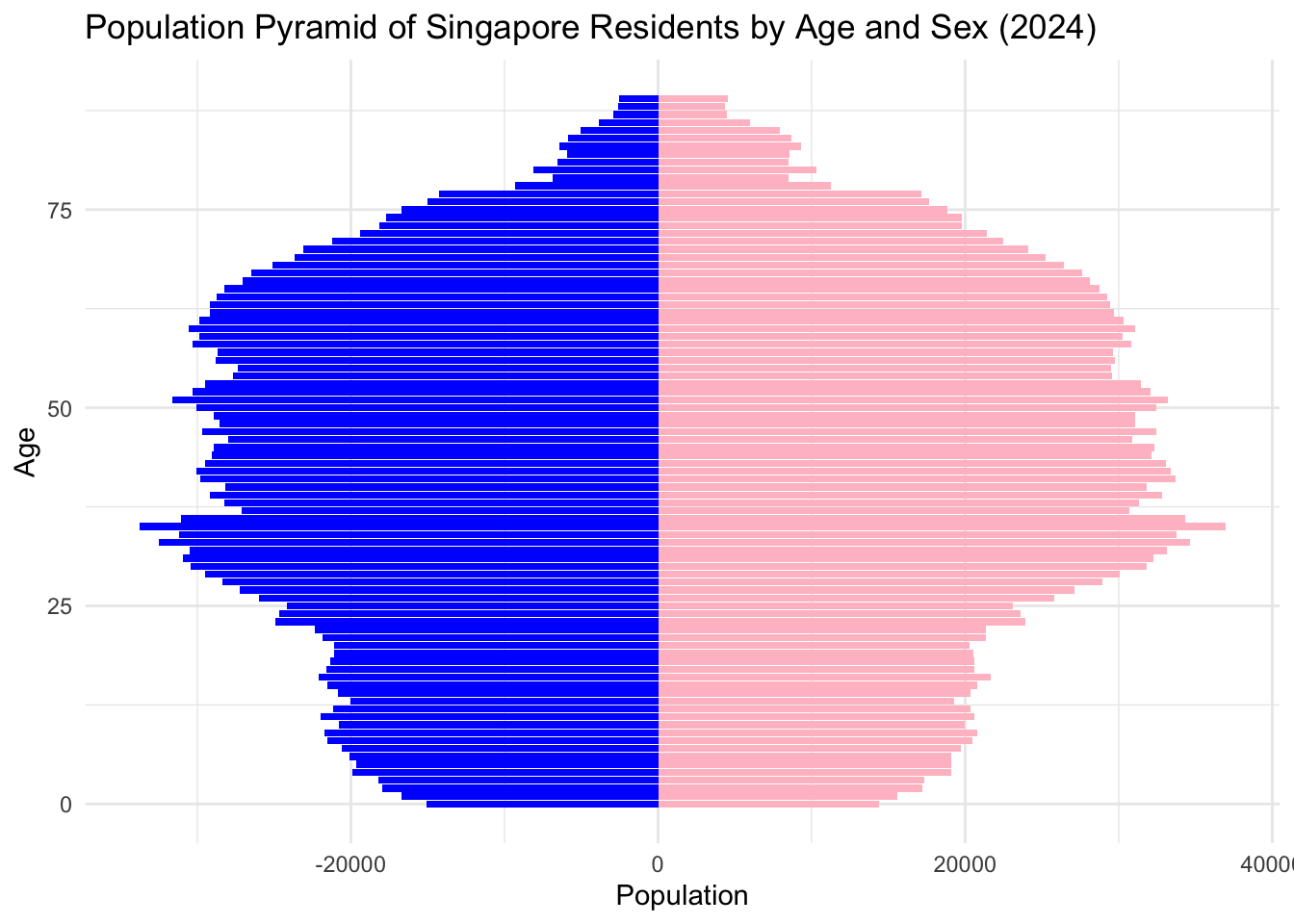

Interpretation:
Aging trend is evident with a large senior population. Strong working-age base from 25–64. Balanced gender distribution across age groups.

4.2 Total Population by Planning Area

pop_area <- df %>%
  group_by(PA) %>%
  summarise(Pop = sum(Pop)) %>%
  arrange(desc(Pop))

ggplot(pop_area, aes(x = reorder(PA, Pop), y = Pop)) +
  geom_col(fill = "steelblue") +
  coord_flip() +
  labs(title = "Total Population by Planning Area (2024)",
       x = "Planning Area", y = "Population") +
  theme_minimal()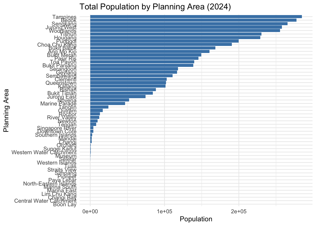

Interpretation:
Planning areas like Bedok, Tampines, and Jurong West are the most populous. Central areas are less populated but may contain older demographics.

4.3 Senior Population Proportion (65+) by Planning Area

senior_df <- df %>%
  group_by(PA, Age) %>%
  summarise(Pop = sum(Pop), .groups = 'drop') %>%
  mutate(AgeGroup = if_else(Age >= 65, "Senior", "Non-Senior")) %>%
  group_by(PA, AgeGroup) %>%
  summarise(Pop = sum(Pop), .groups = 'drop') %>%
  pivot_wider(names_from = AgeGroup, values_from = Pop, values_fill = 0) %>%
  mutate(Senior_Pct = Senior / (Senior + `Non-Senior`) * 100)

ggplot(senior_df, aes(x = reorder(PA, Senior_Pct), y = Senior_Pct)) +
  geom_col(fill = "darkred") +
  coord_flip() +
  labs(title = "Proportion of Seniors (65+) by Planning Area (2024)",
       x = "Planning Area", y = "Senior Population (%)") +
  theme_minimal()

Warning: Removed 13 rows containing missing values or values outside the scale range
(`geom_col()`).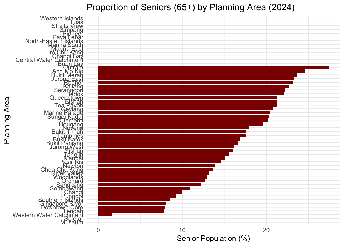

Interpretation:
Central areas like Bukit Merah and Outram have a high proportion of elderly residents, demanding targeted services for aging populations.

4.4 Singapore Population Distribution by Age Group (2024)

age_group_dist <- df %>%
  group_by(AgeGroup) %>%
  summarise(Pop = sum(Pop))

ggplot(age_group_dist, aes(x = AgeGroup, y = Pop)) +
  geom_col(fill = "skyblue") +
  labs(title = "Singapore Population Distribution by Age Group (2024)",
       x = "Age Group", y = "Population") +
  theme_minimal()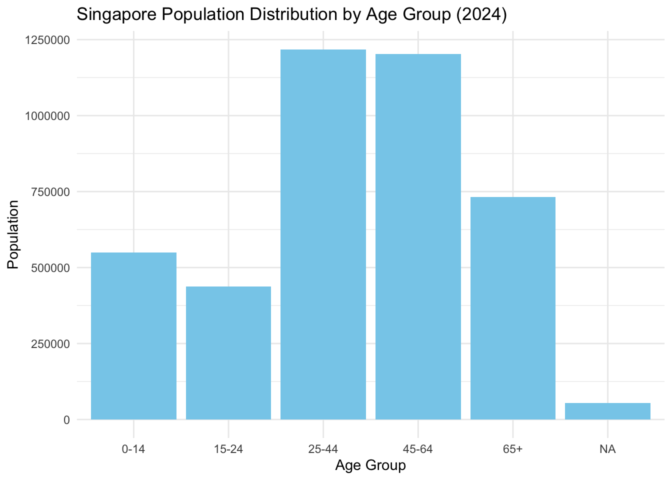

Interpretation:
Working-age groups (25–64) dominate, with growing numbers in the 65+ category. Young children and teens are a smaller share.

4.5 Top 10 Most Populated Subzones (2024)

top_subzones <- df %>%
  group_by(PA, SZ) %>%
  summarise(Pop = sum(Pop), .groups = "drop") %>%
  slice_max(Pop, n = 10)

ggplot(top_subzones, aes(x = Pop, y = fct_reorder(SZ, Pop), fill = PA)) +
  geom_col() +
  labs(title = "Top 10 Most Populated Subzones (2024)",
       x = "Population", y = "Subzone") +
  theme_minimal()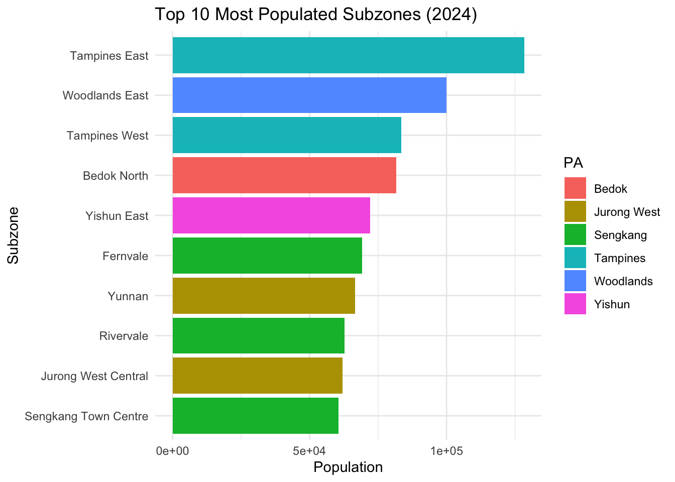

Interpretation:
Subzones in Jurong West, Tampines, and Woodlands are the most densely populated, likely requiring greater investment in local infrastructure.

4.6 Population Heatmap by Planning Area and Age Group (2024)

heatmap_df <- df %>%
  group_by(PA, AgeGroup) %>%
  summarise(Pop = sum(Pop), .groups = "drop") %>%
  pivot_wider(names_from = AgeGroup, values_from = Pop, values_fill = 0)

heatmap_df %>%
  pivot_longer(-PA, names_to = "AgeGroup", values_to = "Pop") %>%
  ggplot(aes(x = AgeGroup, y = PA, fill = Pop)) +
  geom_tile(color = "white") +
  scale_fill_viridis_c() +
  labs(title = "Population Heatmap by Planning Area and Age Group (2024)",
       x = "Age Group", y = "Planning Area") +
  theme_minimal()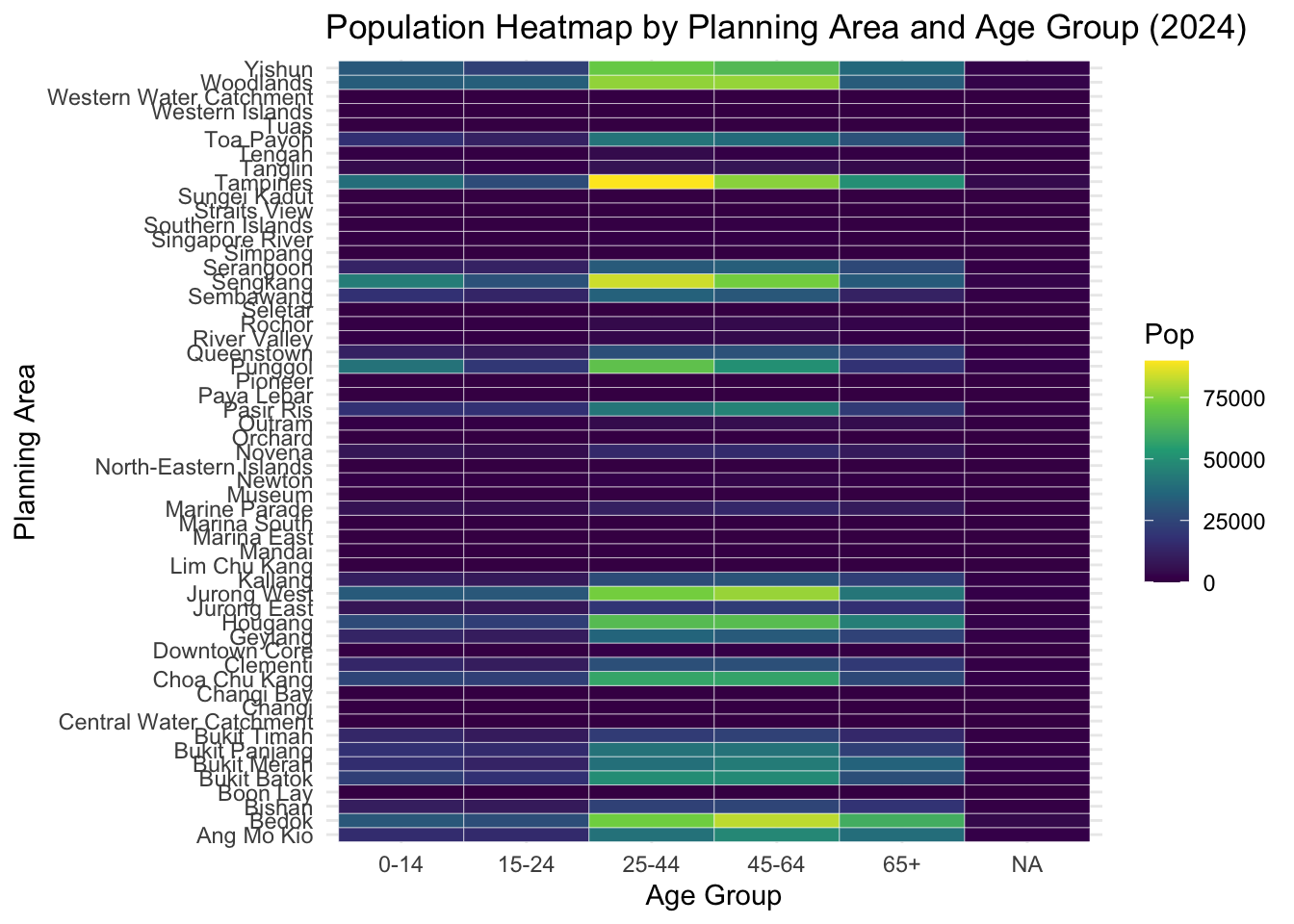

Interpretation:
This matrix highlights how different age groups are distributed. Young clusters in Sengkang and Punggol; older residents dominate central areas.

5. Statistical Summary

summary_df <- df %>%
  group_by(PA) %>%
  summarise(
    Median_Age = median(Age, na.rm = TRUE),
    Elderly_Pct = sum(Pop[Age >= 65], na.rm = TRUE) / sum(Pop, na.rm = TRUE) * 100
  ) %>%
  left_join(
    df %>%
      group_by(PA, SZ) %>%
      summarise(Pop = sum(Pop), .groups = "drop") %>%
      group_by(PA) %>%
      summarise(CV = sd(Pop) / mean(Pop), .groups = "drop"),
    by = "PA"
  )

knitr::kable(summary_df, digits = 2, caption = "Demographic Statistics by Planning Area")

Demographic Statistics by Planning Area
PA	Median_Age	Elderly_Pct	CV
Ang Mo Kio	44.5	24.31	0.77
Bedok	44.5	21.89	0.68
Bishan	44.5	21.07	0.07
Boon Lay	44.5	NaN	NaN
Bukit Batok	44.5	16.72	0.41
Bukit Merah	44.5	23.37	0.63
Bukit Panjang	44.5	16.52	0.50
Bukit Timah	44.5	17.40	0.52
Central Water Catchment	44.5	NaN	NA
Changi	44.5	9.84	1.13
Changi Bay	44.5	NaN	NA
Choa Chu Kang	44.5	13.66	0.23
Clementi	44.5	20.07	0.85
Downtown Core	44.5	7.91	1.61
Geylang	44.5	20.58	0.72
Hougang	44.5	19.51	0.78
Jurong East	44.5	23.13	1.40
Jurong West	44.5	16.12	0.96
Kallang	44.5	22.47	0.94
Lim Chu Kang	44.5	NaN	NA
Mandai	44.5	15.02	1.73
Marina East	44.5	NaN	NA
Marina South	44.5	NaN	NA
Marine Parade	44.5	20.15	1.18
Museum	44.5	0.00	1.54
Newton	44.5	13.82	1.06
North-Eastern Islands	44.5	NaN	NA
Novena	44.5	17.70	1.26
Orchard	44.5	12.64	0.84
Outram	44.5	26.88	1.08
Pasir Ris	44.5	14.51	1.06
Paya Lebar	44.5	NaN	NaN
Pioneer	44.5	NaN	NaN
Punggol	44.5	9.22	0.84
Queenstown	44.5	21.05	1.07
River Valley	44.5	13.12	0.65
Rochor	44.5	22.78	0.93
Seletar	44.5	0.00	2.00
Sembawang	44.5	10.87	1.08
Sengkang	44.5	12.25	0.79
Serangoon	44.5	22.05	0.69
Simpang	44.5	NaN	NaN
Singapore River	44.5	8.10	1.73
Southern Islands	44.5	8.53	1.41
Straits View	44.5	NaN	NA
Sungei Kadut	44.5	20.00	2.24
Tampines	44.5	17.44	0.87
Tanglin	44.5	15.44	0.65
Tengah	44.5	7.81	2.39
Toa Payoh	44.5	21.02	0.54
Tuas	44.5	NaN	NaN
Western Islands	44.5	NaN	NaN
Western Water Catchment	44.5	1.69	1.73
Woodlands	44.5	12.84	1.12
Yishun	44.5	16.01	0.97

Interpretation:
This table shows: - Median Age: Areas like Bedok and Ang Mo Kio have older populations. - Elderly %: Downtown and Bukit Merah have over 20% elderly. - CV (Spread): Population in some PAs is unevenly distributed across subzones, indicating potential resource imbalances.

Key Observations:

Eastern and Northern population hotspots:
Planning areas like Tampines, Bedok, and Sengkang show the highest residential concentrations.
Lower density in central/southern regions:
Marina South, Central Water Catchment, and Downtown Core show low population due to commercial zoning or conservation land use.
Suburban growth in the West and North-West:
Areas like Jurong West and Woodlands reflect continued public housing expansion and decentralised urban planning.
Strategic implications:
Infrastructure, healthcare, and education planning should prioritise high-density residential zones. Meanwhile, low-population regions align with Singapore’s mixed-use and green space strategies.
Uneven population distribution:
The map highlights strong clustering of residential population, aligned with intentional zoning and national development policy.

6. References

Department of Statistics Singapore, 2024 dataset
Kam, T.S. (2023). R for Visual Analytics
Wong, K. (2020). Visual Analytics Course Notes