Hands-on Exercise 4: Visual Statistical Analysis

1. Importing Data

# Read in the Exam.csv file
exam <- read_csv("/Users/sharon/OneDrive - Singapore Management University/isss608data/hands-on_exercise2/Exam_data.csv")

Rows: 322 Columns: 7
── Column specification ────────────────────────────────────────────────────────
Delimiter: ","
chr (4): ID, CLASS, GENDER, RACE
dbl (3): ENGLISH, MATHS, SCIENCE

ℹ Use `spec()` to retrieve the full column specification for this data.
ℹ Specify the column types or set `show_col_types = FALSE` to quiet this message.

# View the structure of the dataset
glimpse(exam)

Rows: 322
Columns: 7
$ ID      <chr> "Student321", "Student305", "Student289", "Student227", "Stude…
$ CLASS   <chr> "3I", "3I", "3H", "3F", "3I", "3I", "3I", "3I", "3I", "3H", "3…
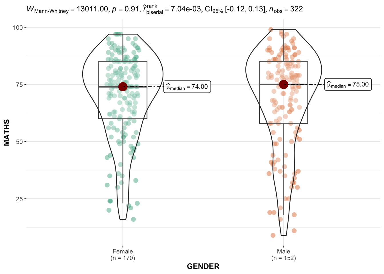
$ GENDER  <chr> "Male", "Female", "Male", "Male", "Male", "Female", "Male", "M…
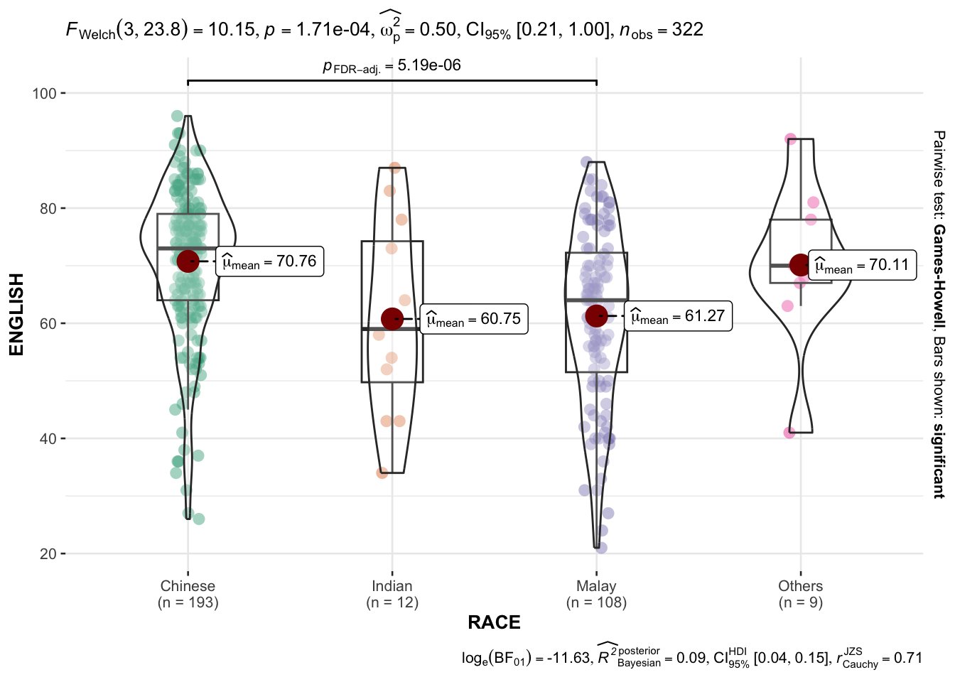
$ RACE    <chr> "Malay", "Malay", "Chinese", "Chinese", "Malay", "Malay", "Chi…
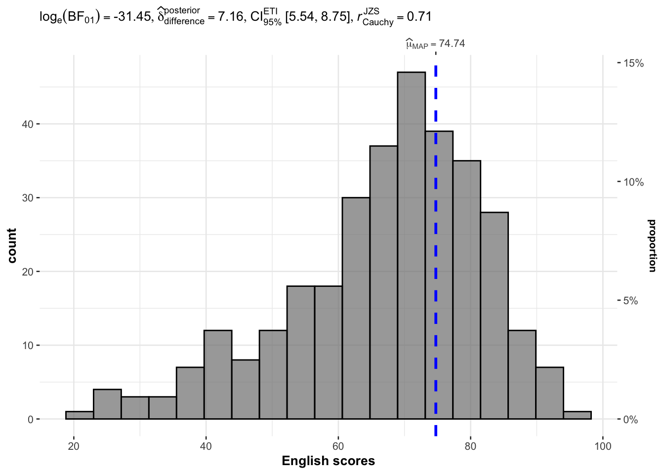
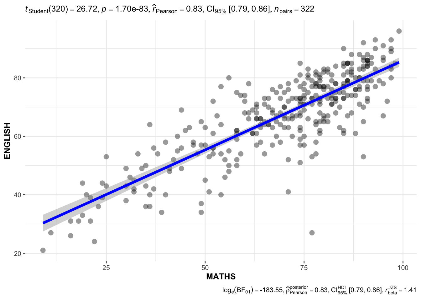
$ ENGLISH <dbl> 21, 24, 26, 27, 27, 31, 31, 31, 33, 34, 34, 36, 36, 36, 37, 38…
$ MATHS   <dbl> 9, 22, 16, 77, 11, 16, 21, 18, 19, 49, 39, 35, 23, 36, 49, 30,…
$ SCIENCE <dbl> 15, 16, 16, 31, 25, 16, 25, 27, 15, 37, 42, 22, 32, 36, 35, 45…

2. One-Sample Test on English Scores

# Visualizing a Bayesian one-sample test for English scores
set.seed(1234)

gghistostats(
  data = exam,
  x = ENGLISH,
  type = "bayes",
  test.value = 60,
  xlab = "English scores"
)

3. Interpreting Bayes Factor

The Bayes Factor (BF10) quantifies the evidence for the alternative hypothesis (H1) compared to the null hypothesis (H0). Interpretation based on Jeffreys’ scale:

BF < 1: Evidence for H0
1 < BF < 3: Anecdotal evidence for H1
3 < BF < 10: Moderate evidence for H1
BF > 10: Strong evidence for H1

4. Two-Sample Mean Test: Maths Scores by Gender

# Visualizing a non-parametric test for Maths scores by Gender
ggbetweenstats(
  data = exam,
  x = GENDER, 
  y = MATHS,
  type = "np",
  messages = FALSE
)

5. One-Way ANOVA Test: English Scores by Race

# One-way ANOVA with post-hoc pairwise comparisons for English scores by Race
ggbetweenstats(
  data = exam,
  x = RACE, 
  y = ENGLISH,
  type = "p",
  mean.ci = TRUE, 
  pairwise.comparisons = TRUE, 
  pairwise.display = "s",
  p.adjust.method = "fdr",
  messages = FALSE
)

6. Correlation Test: Maths vs English Scores

# Visual test of correlation between Maths and English scores
ggscatterstats(
  data = exam,
  x = MATHS,
  y = ENGLISH,
  marginal = FALSE
)

7. Test of Association: Binned Maths Scores vs Gender

# Create bins for Maths scores
exam1 <- exam %>% 
  mutate(MATHS_bins = cut(MATHS, breaks = c(0, 60, 75, 85, 100)))

# Association test between binned Maths scores and Gender
ggbarstats(
  data = exam1, 
  x = MATHS_bins, 
  y = GENDER
)